Testing background point generation in modleR
Andrea Sánchez-Tapia & Sara Mortara
2023-08-03
Source:vignettes/articles/buffer_and_randomPoints.Rmd
buffer_and_randomPoints.RmdThis workflow tests background point generation in
modleR. We perform tests with different types of buffer and
different code options to sample pseudoabsences inside a geographic
buffer. Later, we explore how different methods for sampling
pseudoabsences result on different model predictions.
To run this example you will need modleRand the
additional packages rJava, raster, and
dplyr. To check if they are already installed and install
eventually missing packages run the code below.
packages <- c("rJava", "raster", "dplyr", "devtools")
instpack <- packages[!packages %in% installed.packages()]
if (length(instpack) > 0) {
    install.packages(packages[!packages %in% installed.packages()])
}
If you don’t have modleR installed, run:
Then, load all required packages.
The example data set
We use a standard dataset inside the package modleR.
First, from example_occs object we select only data from
one species Abarema langsdorffii and create one training set
(70% of the data) and one test set (30% of the data) for the data.
## Creating an object with species names
especies <- names(example_occs)[1]
# Selecting only coordinates for the first species
coord1sp <- example_occs[[1]]
head(coord1sp)
## sp lon lat
## 343 Abarema_langsdorffii -40.615 -19.921
## 344 Abarema_langsdorffii -40.729 -20.016
## 345 Abarema_langsdorffii -41.174 -20.303
## 346 Abarema_langsdorffii -41.740 -20.493
## 347 Abarema_langsdorffii -42.482 -20.701
## 348 Abarema_langsdorffii -40.855 -17.082
dim(coord1sp)## [1] 104 3
# Subsetting data into training and test
# Making a sample of 70% of species' records
set <- sample(1:nrow(coord1sp), size = ceiling(0.7 * nrow(coord1sp)))
# Creating training data set (70% of species' records)
train_set <- coord1sp[set,]
# Creating test data set (other 30%)
test_set <- coord1sp[setdiff(1:nrow(coord1sp),set),]
Now let’s the check our data points. We plot the traning and test
data sets with the first axis of the environmental PCA data from the
object example_vars.
# selecting only the first PCA axis
predictor <- example_vars[[1]]
# transforming the data frame with the coordinates in a spatial object
pts <- SpatialPoints(coord1sp[,c(2,3)])
# ploting environmental layer
plot(predictor, legend = FALSE)
# adding training data set in red
points(train_set[,2:3], col = "red", pch = 19)
# adding test data set in blue
points(test_set[,2:3], col = "blue", pch = 19)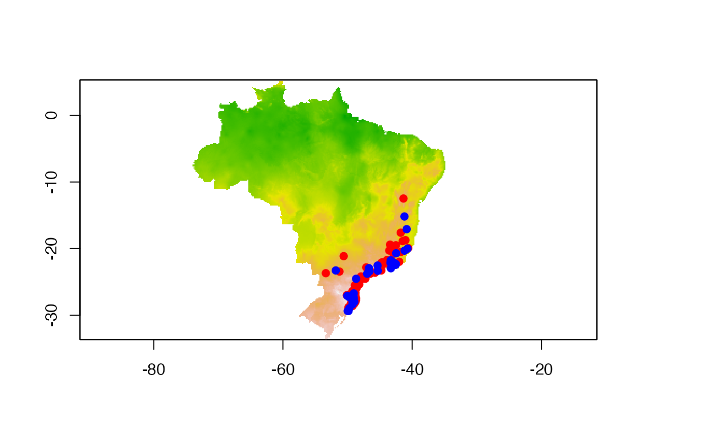
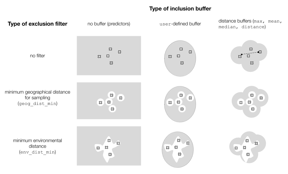
Inclusion buffers (distance-base or user-defined)
We define a buffer as a maximum distance or area, within which pseudoabsences will be sampled. On the other hand, a filter excludes areas too close to the occurrence points (in the environmental or the geographic space), in order to control overfitting.
Here, for all types of buffer and filters, we demonstrate how
function create_buffer() works by running it and then
generating the background values with randomPoints() from
package dismo.
In modleR, we implemented:
- User-defined buffer — Allows the user to provide their own shapefile as available area (M) to sample pseudoabsences
- Geographic distance buffers — Instead of using a specific polygon
for the buffer construction, it samples pseudoabsences according to
several options:
-
max: the maximum distance between any two occurrence points -
mean: the mean distance between all occurrence points -
median: the median of the pairwise distance between occurrence points -
distance: the user can specify a particular distance to be used as buffer width - in raster units
-
- Distance exclusion filters:
- In the geographic space, using parameter
min_geog_dist. - In the environmental space, using
min_env_distand setting adist_type
- In the geographic space, using parameter
Figure 1 explains the possible combinations of these two kinds of buffers.
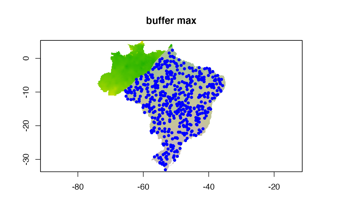
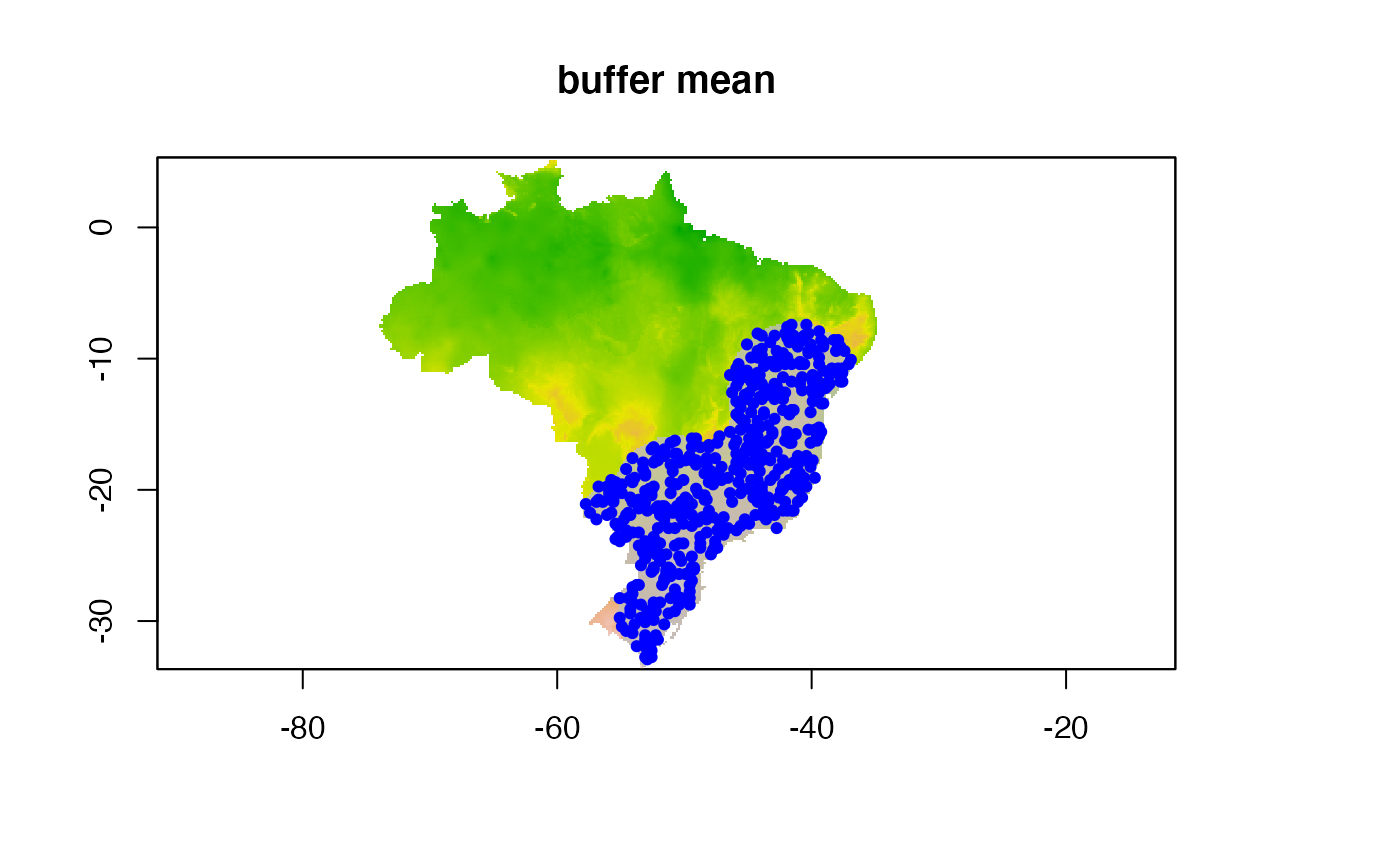
Inclusion buffer with maximum distance max
In this example, we use buffer_type = "maximum" to
generate our first object.

Inclusion buffer with a specific distance
In this example we specify a particular distance from each point to
sample pseudoabsences inside the buffer. We use
buffer_type = "distance" and dist_buf = 5. Be
aware that dist_buf must be set when using a distance
buffer.

Inclusion buffer within a user-defined shapefile (user
and buffer_shape)
In this example we specify a shapefile that we use as the buffer.
Please note that a buffer_shape must be included in order
to use this buffer.
#myshapefile <- rgdal::readOGR("./vignettes/articles/data/myshapefile.shp")
myshapefile <- rgdal::readOGR("./data/myshapefile.shp")
## OGR data source with driver: ESRI Shapefile
## Source: "/Users/andreasancheztapia/Documents/2_proyectos/2_modleR/1_repos_modleR/1_modleR/vignettes/articles/data/myshapefile.shp", layer: "myshapefile"
## with 1 features
## It has 1 fields
buf.user <- create_buffer(occurrences = coord1sp[,c(2,3)],
                          predictors = predictor,
                          buffer_type = "user",
                          buffer_shape = myshapefile)
# using buf.dist to generate 500 pseudoabsences
buf.user.p <- dismo::randomPoints(buf.user,
                                  n = 500,
                                  excludep = TRUE,
                                  p = pts)
# plotting environmental layer with background values
## environmental layer
plot(predictor,
     legend = FALSE, main = "user-defined buffer")
## adding buff
plot(buf.user, add = TRUE, legend = FALSE,
     col = scales::alpha("grey", 0.8), border = "black")
## adding buf.user.p
points(buf.user.p, col = "blue", pch = 19, cex = 0.7)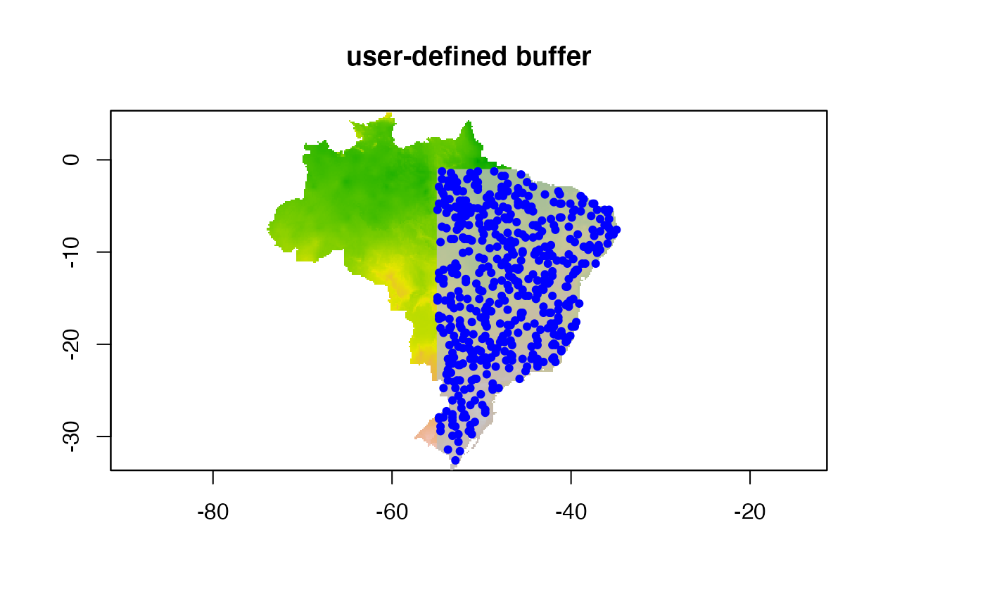
Exclusion filters in the geographical and environmental spaces
Geographic distance filter
The simplest exclusion filter is based on the geographical distance, in the units of the predictor rasters (here, degrees)
geog.filt <- create_buffer(occurrences = coord1sp[,c(2,3)],
                          predictors = predictor,
                          buffer_type = "none",
                          min_geog_dist = 1)

# using buf.dist to generate 500 pseudoabsences
geog.filt.p <- dismo::randomPoints(geog.filt,
                                  n = 500,
                                  excludep = TRUE,
                                  p = pts)
# plotting environmental layer with background values
## environmental layer
plot(predictor,
     legend = FALSE, main = "geographic filter")
## adding buff
plot(geog.filt, add = TRUE, legend = FALSE,
     col = scales::alpha("grey", 0.8), border = "black")
## adding buf.user.p
points(geog.filt.p, col = "blue", pch = 19, cex = 0.7)
points(coord1sp[,c(2,3)], col = "red", pch = 19, cex = 0.7)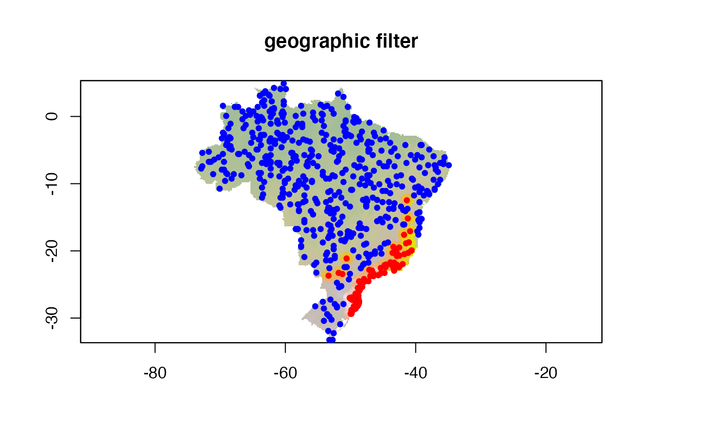
Environmental distance filter
The second kind of filter is based on the euclidean environmental
distance. This can be either the euclidean distance to the environmental
centroid of the occurrences (env_distance = "centroid") or
the minimum euclidean distance to any occurrence point
(env_distance = "mindist").
An example with centroid, taking away 10% of the
closest points
predictor <- example_vars
buf.env <- create_buffer(occurrences = coord1sp[,c(2,3)],
                         predictors = predictor,
                         env_filter = TRUE,
                         env_distance = "centroid",
                         min_env_dist = 0.1
                         )

# using buf.env to generate 500 pseudoabsences
buf.env.p <- dismo::randomPoints(buf.env,
                                  n = 500,
                                  excludep = TRUE,
                                  p = pts)
# plotting environmental layer with background values
## environmental layer
plot(predictor[[1]],
     legend = FALSE, main = "environmental distance filter (centroid)")
## adding buff
plot(buf.env[[1]], add = TRUE, legend = FALSE,
     col = scales::alpha("grey", 0.8), border = "black")
## adding buf.user.p
points(coord1sp[,c(2,3)], col = "red", pch = 19, cex = 0.7)
points(buf.env.p, col = "blue", pch = 19)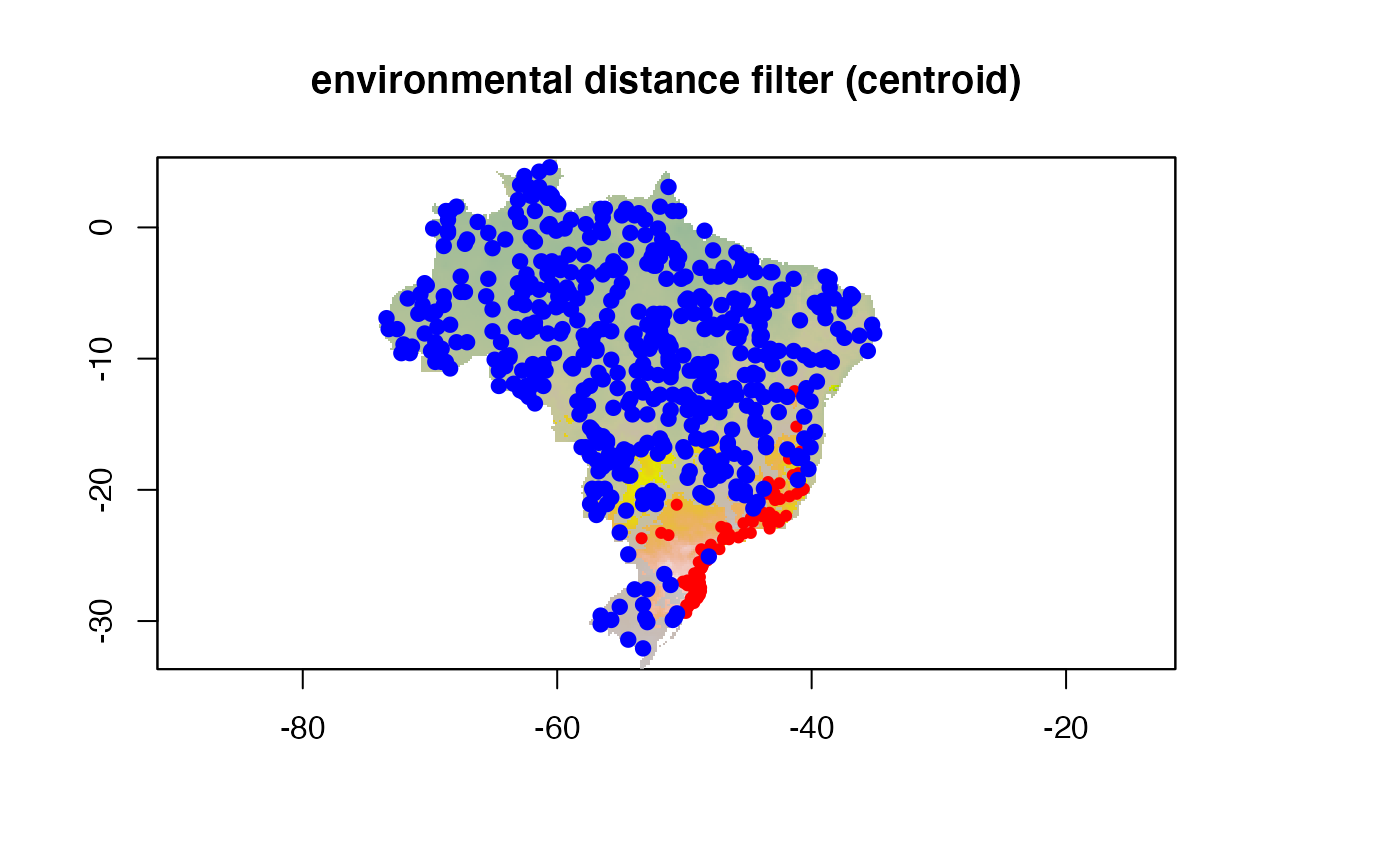
An example with mindist, taking away 10% of the closest
points
predictor <- example_vars
buf.env <- create_buffer(occurrences = coord1sp[,c(2,3)],
                         predictors = predictor,
                         env_filter = TRUE,
                         env_distance = "mindist",
                         min_env_dist = 0.1
                         )

# using buf.env to generate 500 pseudoabsences
buf.env.p <- dismo::randomPoints(buf.env,
                                  n = 500,
                                  excludep = TRUE,
                                  p = pts)
# plotting environmental layer with background values
## environmental layer
plot(predictor[[1]],
     legend = FALSE, main = "environmental distance filter (mindist)")
## adding buff
plot(buf.env[[1]], add = TRUE, legend = FALSE,
     col = scales::alpha("grey", 0.8), border = "black")
## adding buf.user.p
points(coord1sp[,c(2,3)], col = "red", pch = 19, cex = 0.7)
points(buf.env.p, col = "blue", pch = 19)
Superimposing buffers and filters
Buffers and filters can be used simultaneously. Here is an example with a maximum distance buffer and a 5% centroid environmental filter:
buf.env <- create_buffer(occurrences = coord1sp[,c(2,3)],
                         predictors = predictor,
                         buffer_type = "maximum",
                         env_filter = TRUE,
                         env_distance = "centroid",
                         min_env_dist = 0.05)

# using buf.env to generate 500 pseudoabsences
buf.env.p <- dismo::randomPoints(buf.env,
                                  n = 500,
                                  excludep = TRUE,
                                  p = pts)
# plotting environmental layer with background values
## environmental layer
plot(predictor[[1]],
     legend = FALSE, main = "environmental distance buffer x maximum distance buffer")
## adding buff
plot(buf.env, add = TRUE, legend = FALSE,
     col = scales::alpha("grey", 0.8), border = "black")
## adding buf.user.p
points(buf.env.p, col = "blue", pch = 19)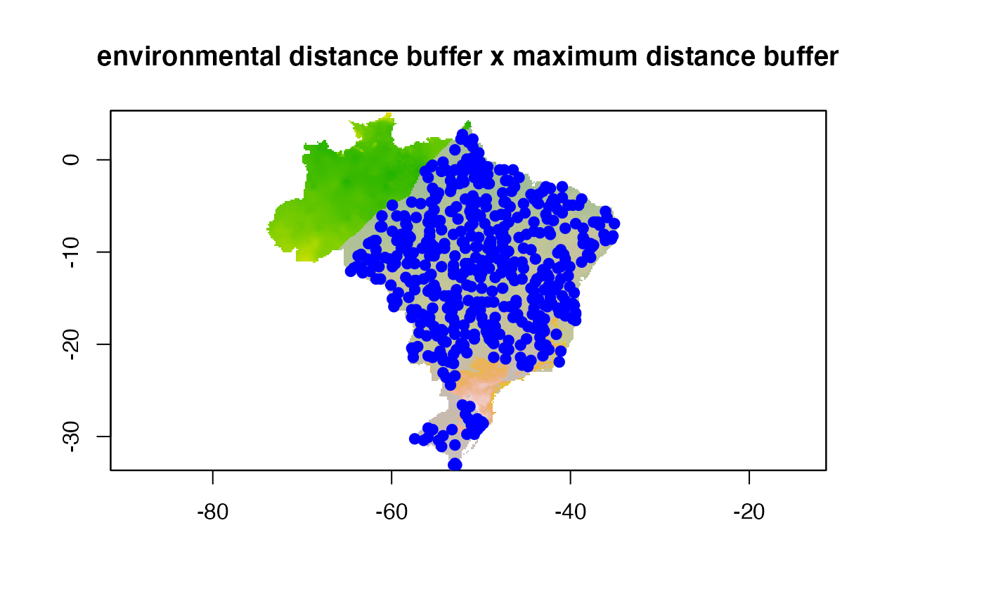
Using function setup_sdmdata()
So far, the examples have been using function
create_buffer() and sampling directly. In modleR, however,
function setup_sdmdata() can take all arguments and execute
the pseudoabsence sampling, as well as data partitioning.
The following examples show the use of function
setup_sdmdata() in several combinations of buffers and
filters.
#maxbuff + mindist
m <- setup_sdmdata(species_name = especies[1],
occurrences = coord1sp[, -1],
predictors = example_vars,
models_dir = "./buffer_res/mindist_maxdist",
buffer_type = "maximum",
min_geog_dist = 3,
clean_dupl = TRUE,
clean_nas = TRUE)
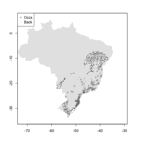
knitr::include_graphics("./buffer_res/mindist_maxdist/Abarema_langsdorffii/present/data_setup/sdmdata_Abarema_langsdorffii.png")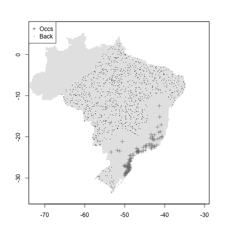
#mean + mindist
m <- setup_sdmdata(species_name = especies[1],
              occurrences = coord1sp[, -1],
              predictors = example_vars,
              models_dir = "./buffer_res/mindist_meandist",
              buffer_type = "mean",
              min_geog_dist = 3,
              clean_dupl = TRUE,
              clean_nas = TRUE)
knitr::include_graphics("./buffer_res/mindist_meandist/Abarema_langsdorffii/present/data_setup/sdmdata_Abarema_langsdorffii.png")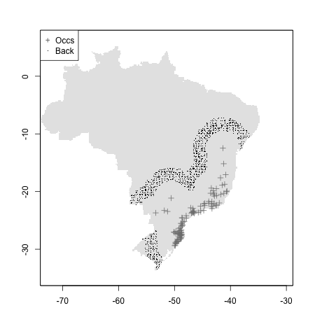
#median + mindist
m <- setup_sdmdata(species_name = especies[1],
              occurrences = coord1sp[, -1],
              predictors = example_vars,
              models_dir = "./buffer_res/mindist_mediandist",
              buffer_type = "median",
              min_geog_dist = 3,
              clean_dupl = TRUE,
              clean_nas = TRUE)
knitr::include_graphics("./buffer_res/mindist_mediandist/Abarema_langsdorffii/present/data_setup/sdmdata_Abarema_langsdorffii.png")
#geog.distance + mindist
m <- setup_sdmdata(species_name = especies[1],
              occurrences = coord1sp[, -1],
              predictors = example_vars,
              models_dir = "./buffer_res/mindist_distance",
              buffer_type = "distance",
              dist_buf = 7,
              min_geog_dist = 3,
              clean_dupl = TRUE,
              clean_nas = TRUE
              )
knitr::include_graphics("./buffer_res/mindist_distance/Abarema_langsdorffii/present/data_setup/sdmdata_Abarema_langsdorffii.png")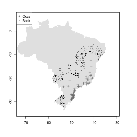
#user + mindist
myshapefile <- rgdal::readOGR("./data/myshapefile.shp")
## OGR data source with driver: ESRI Shapefile
## Source: "/Users/andreasancheztapia/Documents/2_proyectos/2_modleR/1_repos_modleR/1_modleR/vignettes/articles/data/myshapefile.shp", layer: "myshapefile"
## with 1 features
## It has 1 fields
m <- setup_sdmdata(species_name = especies[1],
              occurrences = coord1sp[, -1],
              predictors = example_vars,
              models_dir = "./buffer_res/mindist_usrshp",
              buffer_type = "user",
              buffer_shape = myshapefile,
              min_geog_dist = 3,
              clean_dupl = TRUE,
              clean_nas = TRUE)
knitr::include_graphics("./buffer_res/mindist_usrshp/Abarema_langsdorffii/present/data_setup/sdmdata_Abarema_langsdorffii.png")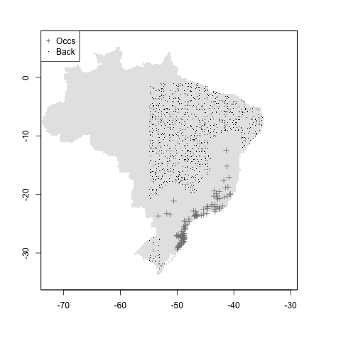
#ENV + mindist
m <- setup_sdmdata(species_name = especies[1],
                   occurrences = coord1sp[, -1],
                   predictors = example_vars,
                   models_dir = "./buffer_res/envdist_usrshp",
                   buffer_type = "mean",
                   env_filter = TRUE,
                   min_env_dist = 0.3,
                   clean_dupl = TRUE,
                   clean_nas = TRUE)
knitr::include_graphics("./buffer_res/envdist_usrshp/Abarema_langsdorffii/present/data_setup/sdmdata_Abarema_langsdorffii.png")